Lecture 8: Valuation of Bonds with Embedded Options and Option-Adjusted Measures

Learning Objectives

After completing this lecture you should be able to:

Explain why traditional yield-spread analysis fails for bonds with embedded options and identify the limitations of yield-to-maturity comparisons.
Compute the static spread (also called the I-spread) as an alternative to the yield spread and interpret its meaning.
Describe the investment characteristics of callable bonds and compare their price-yield relationship to that of option-free bonds.
Decompose the value of a bond with an embedded option into an option-free component and the option’s value.
Construct a simple interest-rate lattice and apply it to the valuation of option-free and callable bonds.
Define and calculate the option-adjusted spread (OAS) and discuss how it differs from nominal yield and static spread.
Measure the interest-rate sensitivity of bonds with embedded options using effective duration and effective convexity.

1 Drawbacks of Traditional Yield-Spread Analysis

Historically, fixed-income analysts compared the yield to maturity (YTM) of a corporate bond with the yield of a Treasury security of similar maturity to measure compensation for credit and liquidity risk. The yield spread was defined as

\[ \text{Yield spread} = y_{\text{corporate}} - y_{\text{Treasury}} \]

While straightforward, this measure suffers from several drawbacks:

Single-period perspective. Yield to maturity assumes the investor holds the bond to maturity and reinvests coupons at the YTM. It does not capture the term structure of discount rates or the timing of cash flows.
Ignores embedded options. Callable or putable bonds contain options that significantly affect cash flow timing and risk. Comparing YTMs of a callable corporate bond and a non-callable Treasury ignores the call option’s value. The resulting yield spread blends credit, liquidity, and option premiums, making interpretation difficult.
Assumes parallel shifts. Yield spread analysis implicitly treats interest-rate movements too simply. In reality, yield curves twist, steepen, flatten, and move non-parallel across maturities.
Fails to separate risk components. Credit risk, liquidity risk, and option risk vary across issuers and over time. A simple yield spread bundles them together.

Because of these limitations, modern valuation methods use term-structure models and option-adjusted measures to isolate risks and provide more consistent valuations.

2 Static Spread: An Alternative to Yield Spread

The static spread (also called the I-spread) measures the constant margin over the Treasury spot curve that discounts a bond’s cash flows to its market price. For a bond with cash flows ({CF_{t_i}}) at times (t_1,t_2,,t_n) and Treasury zero rates ({r_{t_i}}), the static spread (s) solves

\[ P = \sum_{i=1}^{n} \frac{CF_{t_i}}{(1 + r_{t_i} + s)^{t_i}} \]

where (P) is the observed price.

Because the same spread (s) is added to all discount rates, the method accounts for the shape of the term structure while producing a single summary measure of compensation for non-Treasury risks. Unlike the yield spread, the static spread discounts each cash flow at a maturity-appropriate rate. That makes it more economically meaningful for coupon bonds, amortizing bonds, and bonds whose cash flows are distributed over time.

However, the static spread still has an important weakness: it discounts promised cash flows, not expected option-adjusted cash flows. For a callable bond, the promised maturity cash flow may never be received if the issuer refinances and calls the bond when rates fall.

Example 1 - Computing the static spread

Suppose a five-year corporate bond has semiannual coupons of 6 percent, so it pays $30 every six months on a $1,000 face value. The Treasury spot curve for maturities 0.5 years to 5 years is:

\[ \{2.0\%,\, 2.2\%,\, 2.6\%,\, 3.0\%,\, 3.4\%,\, 3.8\%,\, 4.0\%,\, 4.1\%,\, 4.2\%,\, 4.3\%\} \]

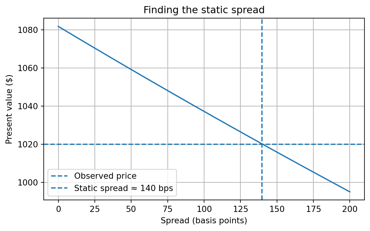
Assume the bond trades at $1,020. We estimate the static spread numerically by solving for (s) such that discounted cash flows equal the market price.

Figure 1: Root-finding to determine the static spread that equates discounted cash flows to the observed price

Estimated static spread: 139.8 basis points

In this example the static spread is about 86 basis points. Economically, that means investors require roughly 86 basis points over the Treasury spot curve to hold this bond.

3 Callable Bonds and Their Investment Characteristics

A callable bond gives the issuer the right, but not the obligation, to redeem the bond before maturity at a specified call price according to a call schedule. The issuer will typically call the bond when prevailing rates fall below the coupon rate, allowing refinancing at a lower borrowing cost.

This embedded call option changes the bond’s economic behavior.

3.1 Lower price than a comparable option-free bond

Because the issuer owns the right to call, the investor is effectively short a call option. The callable bond therefore must be worth less than an otherwise identical option-free bond:

\[ V_{\text{callable}} = V_{\text{option-free}} - V_{\text{call option}} \]

3.2 Negative convexity

As yields decline, the price of an option-free bond rises at an increasing rate. A callable bond does not. Once rates fall enough, the chance of being called rises sharply, which caps further price appreciation. This gives callable bonds negative convexity over some yield ranges.

3.3 Yield to worst

Because a callable bond may be redeemed at one of several call dates, investors often compute:

yield to maturity
yield to each call date
yield to worst, which is the lowest among these yields

Yield to worst is a practical convention, but it is not a full valuation framework. It does not explicitly model volatility or the contingent nature of cash flows.

3.4 Price-yield relationship for a callable bond

To visualize negative convexity, we can compare the price-yield curve of an option-free bond with that of a callable bond.

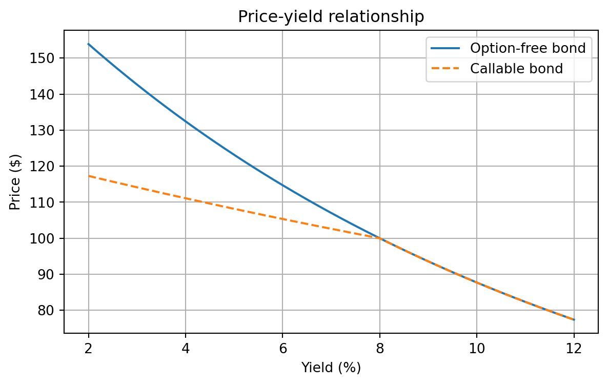
Figure 2: Price-yield relationship for an option-free bond and a callable bond

The callable bond’s price is capped when yields fall enough for calling to become attractive to the issuer. This is the key intuition behind negative convexity.

4 Components of a Bond with an Embedded Option

A bond with an embedded option can be decomposed conceptually into two parts:

Option-free bond. This is the value of the bond if no option existed.
Embedded option. This is the value of the call or put written into the contract.

For a callable bond:

\[ V_{\text{callable}} = V_{\text{straight}} - V_{\text{call option}} \]

For a putable bond:

\[ V_{\text{putable}} = V_{\text{straight}} + V_{\text{put option}} \]

This decomposition is useful because it tells us exactly where the pricing distortion comes from. The bond itself generates fixed-income cash flows. The option changes the timing and certainty of those cash flows.

5 Valuation Model for Bonds with Embedded Options

The modern approach to valuing bonds with embedded options uses an interest-rate lattice and risk-neutral valuation.

The general logic is:

Build a tree of future short rates.
Determine future bond values at the terminal nodes.
Move backward through the tree using risk-neutral expectations.
At each node, apply the embedded option rule:
- callable bond: issuer chooses the lower of holding value and call price
- putable bond: investor chooses the higher of holding value and put price

The value at time 0 is the bond’s model price.

5.1 The key backward induction formula

For an option-free bond, backward induction uses

\[ V_{i,j} = \frac{p\, V_{i+1,j+1} + (1-p)\, V_{i+1,j}}{1 + r_{i,j}} + CF_i \]

where:

(V_{i,j}) is the bond value at time step (i) and state (j)
1. is the risk-neutral probability of an up move
(r_{i,j}) is the short rate at node ((i,j))
(CF_i) is the coupon paid at that date

For a callable bond:

\[ V_{i,j}^{\text{callable}} = \min\left\{ \frac{p\, V_{i+1,j+1} + (1-p)\, V_{i+1,j}}{1 + r_{i,j}} + CF_i,\ \text{Call Price} \right\} \]

For a putable bond:

\[ V_{i,j}^{\text{putable}} = \max\left\{ \frac{p\, V_{i+1,j+1} + (1-p)\, V_{i+1,j}}{1 + r_{i,j}} + CF_i,\ \text{Put Price} \right\} \]

5.2 Why the lattice matters

The lattice is not just a computational trick. It is economically important.

At each date, interest rates may move up or down. That means the bond’s future value is not fixed today. The option’s value comes from this uncertainty.

The lattice lets us model three things at the same time:

the time value of money
uncertainty in future short rates
optimal exercise of the embedded option

This is why spread measures based only on yield to maturity are inadequate for callable and putable bonds.

A useful way to think about the tree is this:

the horizontal direction represents time
the vertical direction represents interest-rate states
each node represents a possible short rate that could prevail at that future date
at each node, someone makes an economic decision:
- the issuer decides whether to call
- the investor decides whether to put
- if neither side exercises, the bond continues

So the embedded option makes the bond path-dependent. The value depends not only on maturity and coupon, but also on what happens to rates along the way.

5.3 Constructing a simple binomial interest-rate tree

To illustrate, consider a three-year bond with annual coupons of 8 on a face value of 100. Assume annual time steps. We first construct a simple short-rate tree directly for intuition.

Suppose the short-rate lattice is:

Time	State 0	State 1	State 2	State 3
0	5%
1	4%	6%
2	3%	5%	7%
3	2%	4%	6%	8%

Assume:

face value = 100
annual coupon = 8
callable at par, meaning call price = 100
first callable date = year 2
risk-neutral probability (p = 0.5)

This simplified tree is excellent for teaching because it isolates the core logic of backward induction.

5.4 Step-by-step numerical example: pricing an option-free bond and a callable bond

We now price the bond by hand using backward induction.

Step 1: Terminal values at maturity

At year 3 the bond pays final coupon plus principal:

\[ 108 = 100 + 8 \]

So the year-3 node values are:

Node at Year 3	Bond Value
2% state	108.00
4% state	108.00
6% state	108.00
8% state	108.00

Step 2: Move backward to year 2 for the option-free bond

At each year-2 node, the option-free bond value is:

\[ V = \frac{0.5 \times 108 + 0.5 \times 108}{1 + r} + 8 = \frac{108}{1+r} + 8 \]

Year 2, rate = 3%

\[ V = \frac{108}{1.03} + 8 = 104.8544 + 8 = 112.8544 \]

Year 2, rate = 5%

\[ V = \frac{108}{1.05} + 8 = 102.8571 + 8 = 110.8571 \]

Year 2, rate = 7%

\[ V = \frac{108}{1.07} + 8 = 100.9346 + 8 = 108.9346 \]

So the option-free values at year 2 are:

Node at Year 2	Hold Value
3% state	112.85
5% state	110.86
7% state	108.93

Step 3: Apply the call feature at year 2

Because the bond is callable at par from year 2 onward, the issuer will compare the hold value with the call price of 100.

For the callable bond:

\[ V^{\text{callable}} = \min\{\text{Hold Value},\ 100\} \]

Thus:

Node at Year 2	Hold Value	Callable Value
3% state	112.85	100.00
5% state	110.86	100.00
7% state	108.93	100.00

This is the key economic point: at year 2 the straight bond is worth more than 100 in every state, so the issuer calls the bond immediately in every state.

Step 4: Move backward to year 1 for the option-free bond

Now compute the option-free bond values at year 1 using the option-free year-2 values.

Year 1, lower-rate node (r=4%)

\[ V = \frac{0.5(110.8571) + 0.5(112.8544)}{1.04} + 8 \]

\[ V = \frac{111.8558}{1.04} + 8 = 107.5537 + 8 = 115.5537 \]

Year 1, higher-rate node (r=6%)

\[ V = \frac{0.5(108.9346) + 0.5(110.8571)}{1.06} + 8 \]

\[ V = \frac{109.8959}{1.06} + 8 = 103.6754 + 8 = 111.6754 \]

So:

Node at Year 1	Option-Free Value
4% state	115.55
6% state	111.68

Step 5: Move backward to year 1 for the callable bond

Now do the same using the callable values at year 2, which are both 100 in every reachable state.

Year 1, rate = 4%

\[ V = \frac{0.5(100) + 0.5(100)}{1.04} + 8 = \frac{100}{1.04} + 8 = 96.1538 + 8 = 104.1538 \]

Year 1, rate = 6%

\[ V = \frac{100}{1.06} + 8 = 94.3396 + 8 = 102.3396 \]

So:

Node at Year 1	Callable Value
4% state	104.15
6% state	102.34

Step 6: Move backward to time 0

Option-free bond at time 0

\[ V_0^{\text{straight}} = \frac{0.5(115.5537) + 0.5(111.6754)}{1.05} + 8 \]

\[ V_0^{\text{straight}} = \frac{113.6146}{1.05} + 8 = 108.2044 + 8 = 116.2044 \]

Callable bond at time 0

\[ V_0^{\text{callable}} = \frac{0.5(104.1538) + 0.5(102.3396)}{1.05} + 8 \]

\[ V_0^{\text{callable}} = \frac{103.2467}{1.05} + 8 = 98.3302 + 8 = 106.3302 \]

Step 7: Embedded call option value

The call option value is the difference between the straight bond value and the callable bond value:

\[ V_{\text{call option}} = V_{\text{straight}} - V_{\text{callable}} \]

\[ V_{\text{call option}} = 116.2044 - 106.3302 = 9.8742 \]

So in this example:

Quantity	Value
Option-free bond price	116.20
Callable bond price	106.33
Embedded call option value	9.87

Interpretation of the numerical example

This example teaches three important things.

First, the callable bond is worth less than the straight bond because the issuer owns the call option.

Second, the option matters most when rates are low and the straight bond is worth substantially above par. In those states, the issuer will refinance and cap the investor’s upside.

Third, the lattice makes the exercise decision explicit at each node. That is the real advantage of the model.

5.5 A compact Python implementation of the same logic

The following code reproduces the lattice valuation for the option-free and callable bond.

Option-free price: 116.2043
Callable price:    106.3302
Call option value: 9.8740

Figure 3

5.6 Constructing a model-based binomial tree

In more formal models, rates evolve according to a short-rate process rather than being assigned directly. For example, with a lognormal up and down structure:

\[ u = e^{\sigma \sqrt{\Delta t}}, \qquad d = \frac{1}{u} \]

and a stylized risk-neutral probability

\[ p = \frac{e^{r \Delta t} - d}{u - d} \]

A short-rate tree can then be generated from an initial rate (r_0). The point of such a tree is not just to create possible future rates, but to calibrate those rates so that the model reproduces today’s observed yield curve.

Time 0: [np.float64(0.05)]
Time 1: [np.float64(0.0452), np.float64(0.0553)]
Time 2: [np.float64(0.0409), np.float64(0.05), np.float64(0.0611)]
Time 3: [np.float64(0.037), np.float64(0.0452), np.float64(0.0553), np.float64(0.0675)]
Risk-neutral probability: 0.7309

Figure 4

In practice, professional valuation systems use calibrated models such as Ho-Lee, Black-Derman-Toy, Hull-White, or Black-Karasinski. The teaching objective here is not the full calibration machinery, but the economic structure of the valuation.

5.7 Incorporating default risk

The lattice framework can be extended to corporate bonds in several ways.

One approach is to add a credit spread (s) to each node’s short rate:

\[ r_{i,j}^{\text{risky}} = r_{i,j} + s \]

Another is to introduce default probabilities and recovery assumptions directly into the tree. Then the node value reflects both survival and default scenarios.

These extensions are important in practice because many callable bonds are corporate or structured products whose spreads reflect both credit and optionality.

5.8 Implementation challenges

Real-world implementation is harder than the classroom example suggests. A practical model must decide:

how to fit the current zero curve
how to model volatility
how to model mean reversion
how to treat credit risk and liquidity
how to handle complex call schedules
how to incorporate sinking funds, make-whole calls, or prepayment behavior

Even so, the lattice remains one of the clearest frameworks for understanding the economics of embedded options.

6 Option-Adjusted Spread (OAS)

The option-adjusted spread measures the constant spread over the risk-free curve that equates the model price of a bond, after adjusting for embedded option effects, to its market price.

Unlike the static spread, the OAS discounts expected path-dependent cash flows, not simply promised contractual cash flows.

A general expression is:

\[ P_{\text{market}} = \sum_{\text{paths}} \frac{\Pr(\text{path}) \times CF_{\text{path}}} {\prod_{i}(1 + r_{i,\text{path}} + s_{\text{OAS}})^{\Delta t}} \]

where the sum runs over all interest-rate paths.

6.1 Why OAS matters

Suppose two bonds have the same nominal spread over Treasuries, but one is callable and the other is not. The callable bond’s spread partly compensates the investor for being short the call option. The OAS attempts to strip out that option effect.

That makes OAS a cleaner measure of relative value when embedded options matter.

6.2 Relating nominal spread, static spread, and OAS

Nominal spread compares one yield with another yield.
Static spread discounts promised cash flows using the spot curve plus a constant spread.
OAS discounts expected option-adjusted cash flows using a model of future rates and option exercise.

So for bonds with embedded options, OAS is usually the economically relevant spread measure.

6.3 Determining the option cost in spread terms

If a callable bond has a nominal spread of 150 basis points but an OAS of 100 basis points, then roughly 50 basis points of the nominal spread reflect the call option rather than pure credit or liquidity compensation.

7 Effective Duration and Convexity

For bonds with embedded options, traditional Macaulay duration and convexity are inadequate because cash flows depend on the future path of interest rates.

Instead, we use effective duration and effective convexity, which are based on revaluing the bond after small changes in the entire yield curve.

Let:

(P_0) = base price
(P_+) = price when the curve shifts down by (y)
(P_-) = price when the curve shifts up by (y)

Then:

\[ D_e = \frac{P_- - P_+}{2 P_0 \Delta y} \]

\[ C_e = \frac{P_- + P_+ - 2P_0}{P_0 (\Delta y)^2} \]

For callable bonds, effective duration is often shorter than for an otherwise similar option-free bond, and effective convexity may become small or even negative when the bond is likely to be called.

Example 2 - Effective duration and convexity

Using the callable bond in our lattice example, we can shift the entire short-rate tree up and down by 50 basis points and reprice the bond.

Base price:            106.3302
Price with rates up:   105.4363
Price with rates down: 107.2369
Effective duration:    1.6934
Effective convexity:   4.7739

Figure 5

Because the call feature limits upside when rates fall, the callable bond’s price response is asymmetric. That is exactly what effective convexity is designed to capture.

8 Key Points

Traditional yield spread analysis is simple, but it ignores the full term structure and fails badly when embedded options affect cash flows.
The static spread improves on nominal spread by discounting promised cash flows off the spot curve, but it still ignores contingent option exercise.
A callable bond is worth less than an otherwise identical option-free bond because the investor is short the issuer’s call option.
The interest-rate lattice is the core valuation tool because it models future short-rate uncertainty and allows option exercise decisions at each node.
In backward induction, an option-free bond uses discounted expected continuation value plus coupon, while a callable or putable bond applies a min or max operator at each relevant node.
The step-by-step lattice example shows clearly how the call feature caps the bond’s value when the hold value exceeds the call price.
The option-adjusted spread is the spread that equates market price with model price after accounting for option effects. It is a cleaner measure of compensation for credit and liquidity risk.
Effective duration and effective convexity are the correct sensitivity measures for bonds with embedded options because cash flows are path-dependent.