Lecture 7: Interest‑Rate Models

Learning Objectives

After completing this lecture you will be able to:

Define an interest‑rate model and interpret its key components (drift, volatility and mean reversion).
Explain the mathematics behind one‑factor stochastic processes used to model interest rates.
Distinguish between arbitrage‑free and equilibrium interest‑rate models and understand the purpose of each.
Discuss empirical evidence on interest‑rate changes, including how volatility relates to rate levels and the possibility of negative rates.
Describe criteria for selecting an interest‑rate model in practice.
Compute historical interest‑rate volatility using real or simulated data.

1 Mathematical Description of One‑Factor Interest‑Rate Models

An interest‑rate model is a probabilistic description of how interest rates evolve over time. In fixed‑income portfolio management, models help value bonds and derivatives and simulate future yield curves. Models must specify how the short‑term rate evolves and how that short rate determines the rest of the term structure.

1.1 A basic continuous‑time stochastic process

In a basic one‑factor model, the short rate \(r_t\) is assumed to follow a stochastic differential equation (SDE) of the form

\[ \mathrm{d}r_t = b\,\mathrm{d}t + \sigma\,\mathrm{d}z_t, \]

where:

\(b\) is the drift term representing the expected direction of the change in the short rate.
\(\sigma\) is the volatility term representing the magnitude of random shocks.
\(z_t\) is a standard Wiener process (Brownian motion).

The drift and volatility are constants in this simplest model. If \(b=0\), the expected change in \(r\) is zero and the variance of the change over a time interval of length \(T\) is \(\sigma^2 T\). Models of this type are sometimes called normal models because rate changes are independent of the current level.

1.2 Itô process

In reality, drift and volatility are not constant; they can depend on the current level of the short rate \(r\) and time \(t\). An Itô process allows this by writing

\[ \mathrm{d}r_t = b(r_t,t)\,\mathrm{d}t + \sigma(r_t,t)\,\mathrm{d}z_t. \]

Here, \(b(r_t,t)\) and \(\sigma(r_t,t)\) can be functions of \(r_t\) and \(t\). Itô processes are the building block of most one‑factor term‑structure models.

1.3 Specifying the dynamics of the drift term

A common specification for the drift is mean reversion. The idea is that interest rates tend to revert toward a long‑run average \(\bar{r}\). The speed of mean reversion is measured by a parameter \(\alpha>0\). The drift becomes

\[ b(r_t,t) = -\alpha\bigl(r_t - \bar{r}\bigr). \]

When \(r_t\) is above the long‑run mean, the drift is negative; when below, it is positive. The speed \(\alpha\) controls how quickly \(r_t\) moves back toward \(\bar{r}\).

1.4 Specifying the dynamics of the volatility term

Volatility can depend on the level of rates. A flexible specification is the constant‑elasticity‑of‑variance (CEV) model, which sets

\[ \sigma(r_t,t) = \sigma_0\,r_t^{\gamma}, \]

where \(\sigma_0>0\) is a scale parameter and \(\gamma\) controls how volatility depends on \(r_t\). Special cases include:

\(\gamma=0\) (Vasicek model): volatility is constant and independent of \(r_t\). This is a normal model.
\(\gamma=1\) (Dothan model): volatility is proportional to \(r_t\). This is a lognormal model (changes are proportional to the level).
\(\gamma=\tfrac{1}{2}\) (Cox–Ingersoll–Ross model): volatility is proportional to \(\sqrt{r_t}\). This avoids negative rates because \(\sigma_0 r_t^{1/2}\) goes to zero as \(r_t\) approaches zero.

Combining mean reversion in drift with square‑root volatility yields the mean‑reverting square‑root model:

\[ \mathrm{d}r_t = -\alpha(r_t-\bar{r})\,\mathrm{d}t + \sigma_0\sqrt{r_t}\,\mathrm{d}z_t. \]

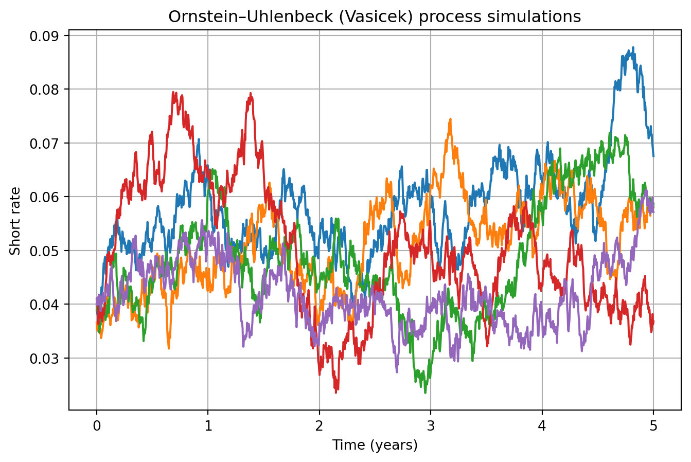
🧮 Example: Simulating an Ornstein–Uhlenbeck process

An Ornstein–Uhlenbeck (Vasicek) process has constant volatility and mean‑reverting drift. The following Python code simulates sample paths:

Figure 1: Simulated short‑rate paths following an Ornstein–Uhlenbeck process

This graph shows sample short‑rate paths reverting toward the long‑run mean.

2 Arbitrage‑Free versus Equilibrium Models

Interest‑rate models can be classified by how they determine the term‑structure evolution.

2.1 Arbitrage‑free models

Arbitrage‑free or no‑arbitrage models start with observed market prices of a set of benchmark instruments (Treasury bonds, swaps, etc.). The model assumes a random process for the short rate with unknown drift. Parameters are calibrated so that the model exactly reproduces the current term structure and prices of benchmark instruments. Once calibrated, the model can value other instruments consistently.

Common arbitrage‑free models include:

Model	Type	Key features
Ho–Lee	Normal	Constant volatility; no mean reversion. Produces normally distributed rate changes.
Hull–White	Normal	Adds mean reversion to the Ho–Lee model. Useful for pricing callable bonds.
Kalotay–Williams–Fabozzi (KWF)	Lognormal	Models the logarithm of the short rate; no mean reversion.
Black–Karasinski	Lognormal	Lognormal model with mean reversion.
Black–Derman–Toy	Lognormal	Lognormal with endogenous mean reversion; calibrates to caps and floors.
Heath–Jarrow–Morton (HJM)	General	Multi‑factor model specifying the volatility structure of forward rates. Many models (Ho–Lee, Hull–White, KWF, etc.) are special cases.

Because these models match observed prices, arbitrage opportunities are eliminated by construction. They are widely used in practice for pricing complex derivatives and bonds with embedded options.

2.2 Equilibrium models

Equilibrium models explain the term structure by appealing to economic fundamentals and investor preferences. They assume a particular utility function and derive the stochastic process for rates from equilibrium conditions. Parameters are estimated from historical data rather than calibrated to market prices. Examples include the Vasicek and Cox–Ingersoll–Ross (CIR) equilibrium models, as well as the Brennan–Schwartz and Longstaff–Schwartz two‑factor models.

Equilibrium models provide economic intuition but are less commonly used to price derivatives because they do not necessarily fit the current term structure. In practice, arbitrage‑free models dominate due to their ability to match observed prices and deliver consistent valuations.

3 Empirical Evidence on Interest‑Rate Changes

When choosing a model, it helps to understand actual interest‑rate behaviour. Two issues are often discussed: the relationship between volatility and the level of rates, and the possibility of negative rates.

3.1 Volatility of rates and the level of interest rates

Empirical studies of Treasury yield curves from the late 1970s to the 2000s show that the correlation between interest‑rate volatility and the level of rates changes across regimes【671527559854124†screenshot】. During periods when rates exceeded roughly 10% (late 1970s and early 1980s), volatility tended to increase with the level of rates. When rates were below 10%, the correlation weakened and volatility behaved more like a constant. This evidence suggests that in low‑rate environments (common since the 1990s), the normal model (constant volatility) may be adequate, whereas in high‑rate regimes a lognormal or square‑root model might better reflect the link between level and volatility.

3.2 Negative interest rates

Historical episodes show that nominal rates can occasionally be negative. During the U.S. Great Depression, Treasury bills traded at negative yields; more recently some short‑term Japanese yen deposits briefly had negative yields in the late 1990s. Models with constant volatility allow negative rates, while models where volatility is proportional to the rate (lognormal) do not. Empirical tests indicate that the probability of negative rates under realistic parameter values is small and has little impact on derivative pricing. Hence, many practitioners are comfortable using normal models even though they admit negative rates.

4 Selecting an Interest‑Rate Model

When choosing a model for bond portfolio management, consider:

Purpose of the model. For pricing complex derivatives or option‑embedded bonds, use arbitrage‑free models that fit the current term structure. For economic insight or macroeconomic forecasting, equilibrium models may suffice.
Volatility assumptions. In low‑rate environments, constant volatility models (Vasicek, Ho–Lee, Hull–White) perform well. In high‑rate regimes or when negative rates must be ruled out, lognormal or square‑root volatility (CIR, Black–Karasinski) may be preferred.
Computational tractability. Models should allow efficient calibration and pricing. Multi‑factor models offer flexibility but are more difficult to implement.
Data availability. Arbitrage‑free models require reliable market prices for a reference set of instruments; equilibrium models require long historical series to estimate parameters.

Ultimately, practitioners often choose the simplest model that fits the current term structure and provides robust valuations across scenarios.

5 Estimating Interest‑Rate Volatility Using Historical Data

Volatility is an important input for any rate model. Two common methods are historical volatility and implied volatility.

5.1 Historical volatility

Historical volatility uses past interest‑rate observations to estimate the standard deviation of rate changes. Suppose \(r_t\) is a series of weekly interest rates and \(\Delta r_t\) is the change from one week to the next. The sample standard deviation of \(\Delta r_t\) provides a weekly volatility. To annualize, multiply by \(\sqrt{52}\) (assuming 52 weeks per year). For daily data, multiply the daily standard deviation by \(\sqrt{n}\), where \(n\) is the number of trading days in a year (commonly 250 or 260).

Numerical example (artificial data)

Consider a hypothetical sequence of weekly short rates (in percent) over 10 weeks:

Week	Rate (%)	Weekly change (\(\Delta r_t\), bps)
1	2.00	–
2	2.05	+5
3	2.04	−1
4	2.08	+4
5	2.02	−6
6	2.10	+8
7	2.09	−1
8	2.12	+3
9	2.15	+3
10	2.14	−1

To compute the sample standard deviation of the changes, convert basis points to decimal form (e.g., +5 bps = 0.0005). Using the eight non‑missing changes (+5, −1, +4, −6, +8, −1, +3, +3, −1) we find:

Mean change = \(\frac{5 - 1 + 4 - 6 + 8 - 1 + 3 + 3 - 1}{9} = \frac{14}{9} \approx 1.556\) bps.
Variance = \(\frac{1}{8}\sum_{i=1}^{9} (\Delta r_i - \text{mean})^2\). Calculating each squared deviation and summing yields \(\approx 94.22\) (bp)\(^2\). The sample variance is \(94.22/8 \approx 11.78\) (bp)\(^2\).
Standard deviation = \(\sqrt{11.78} \approx 3.43\) bps per week.
Annualized volatility = \(3.43 \times \sqrt{52} \approx 24.7\) bps per year.

Thus, this simplified data set implies an annual volatility of about 25 basis points.

The calculation can also be performed programmatically. Below we generate a synthetic time series and compute the historical volatility:

import pandas as pd
import numpy as np
import matplotlib.pyplot as plt

# Create synthetic weekly rates (percent)
rates = np.array([2.00, 2.05, 2.04, 2.08, 2.02, 2.10, 2.09, 2.12, 2.15, 2.14])
changes_bp = (np.diff(rates) * 10000)  # convert percent differences to basis points

# Compute weekly volatility in bps
mean_change = changes_bp.mean()
vol_weekly = changes_bp.std(ddof=1)  # sample standard deviation in bps
vol_annual = vol_weekly * np.sqrt(52)

vol_weekly, vol_annual

(np.float64(418.66188956934894), np.float64(3019.01381984986))

Synthetic weekly rates and computed historical volatility

This code calculates the weekly and annualized volatilities in basis points for the synthetic data. You can modify the rates array to explore different scenarios.

5.2 Implied volatility

Implied volatility derives from market prices of option‑like instruments (caps, floors, swaptions). An option pricing model expresses the option price as a function of volatility. By inverting the model using observed prices, one obtains the market’s expected volatility. Implied volatility reflects current market conditions and forward‑looking expectations, whereas historical volatility reflects past behaviour.

6 Key Points

An interest‑rate model specifies a stochastic process for the short rate and derives other rates from it. Drift, volatility and mean reversion are key components.
One‑factor models use a single source of uncertainty (Brownian motion). Mean‑reverting drift and level‑dependent volatility are common specifications.
Arbitrage‑free models (Ho–Lee, Hull–White, KWF, Black–Karasinski, BDT, HJM) calibrate to market prices and are widely used for valuation. Equilibrium models (Vasicek, CIR, Brennan–Schwartz, Longstaff–Schwartz) derive rates from economic assumptions.
Empirical evidence suggests that volatility is largely independent of the level of rates when rates are below about 10%, supporting the normal model; at higher levels, volatility may increase with rates, favouring lognormal specifications【671527559854124†screenshot】.
Negative nominal rates can occur but are rare. Normal models admit negative rates; the probability of occurrence is small under realistic parameters.
Historical volatility is computed from past rate changes and annualized using square‑root‑of‑time scaling; implied volatility is extracted from option prices.

Suggested readings: Fabozzi, Bond Markets: Analysis and Strategies, Chapter 17.